Your μ Matters: Understanding Turbulence Model Behavior

Author:
Erik Tylczak
Senior Research Engineer

I recently attended an internal Convergent Science advanced training course on turbulence modeling. One of the audience members asked one of my favorite modeling questions, and I’m happy to share it here. It’s the sort of question I sometimes find myself asking tentatively, worried I might have missed something obvious. The question is this:

Reynolds-Averaged Navier Stokes (RANS) turbulence models and Large-Eddy Simulation (LES) turbulence models have very different behavior. LES will become a direct numerical simulation (DNS) in the limit of infinitesimally fine grid, and it shows a wide range of turbulent length scales. RANS does not become a DNS, no matter how fine we make the grid. Rather, it shows grid-convergent behavior (i.e., the simulation results stop changing with finer and finer grids), and it removes small-scale turbulent content.

If I look at a RANS model or an LES turbulence model, the transport equations look very similar mathematically. How does the flow ‘know’ which is which?

There’s a clever, physically intuitive answer to this question, which motivates the development of additional hybrid models. But first we have to do a little bit of math.

Both RANS and LES take the approach of decomposing a turbulent flow into a component to be resolved and a component to be modeled. Let’s define the Reynolds decomposition of a flow variable ϕ as

$$\phi = \bar \phi \; + \;\phi’,$$

where the overbar term represents a time/ensemble average and the prime term is the fluctuating term. This decomposition has the following properties:

$$\overline{\overline{\phi}} = \bar \phi \;\;{\rm{and}}\;\;\overline{\phi’} = 0.$$

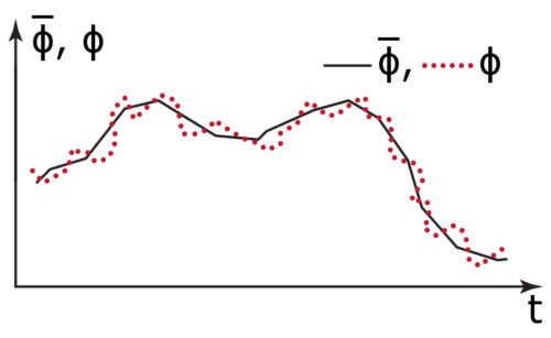
LES uses a different approach, which is a spatial filter. The filtering decomposition of ϕ is defined as

$$\phi  = \left\langle \phi  \right\rangle + \;\phi ”,$$

where the term in the angled brackets is the filtered term and the double-prime term is the sub-grid term. In practice, this is often calculated using a box filter, a spatial average of everything inside, say, a single CFD cell. The spatial filter has different properties than the Reynolds decomposition,

$$\left\langle {\left\langle \phi  \right\rangle } \right\rangle \ne \left\langle \phi  \right\rangle \;\;{\rm{and}}\;\;\left\langle {\phi ”} \right\rangle  \ne 0.$$

To derive RANS and LES turbulence models, we apply these decompositions to the Navier-Stokes equations. For simplicity, let’s consider only the incompressible momentum equation. The Reynolds-averaged momentum equation is written as

$$\frac{{\partial \overline {{u_i}} }}{{\partial t}} + \frac{{\partial \overline {{u_i}}\; \overline {{u_j}} }}{{\partial {x_j}}} = – \frac{1}{\rho }\frac{{\partial \overline P }}{{\partial {x_i}}} + \frac{1}{\rho }\frac{\partial }{{\partial {x_j}}}\left[ {\mu \left( {\frac{{\partial \overline {{u_i}} }}{{\partial {x_j}}} + \frac{{\partial \overline {{u_j}} }}{{\partial {x_i}}}} \right) – \frac{2}{3}\mu \frac{{\partial \overline {{u_k}} }}{{\partial {x_k}}}{\delta _{ij}}} \right] – \frac{1}{\rho }\frac{\partial }{{\partial {x_j}}}\left( {\rho \color{Red}{\overline {{{u’}_i}{{u’}_j}}} } \right).$$

This equation looks the same as the basic momentum transport equation, replacing each variable with the barred equivalent, with the exception of the term* in red. That’s where the RANS model will make a contribution.

The LES momentum equation, again neglecting Favre filtering, is written

$$\frac{{\partial \left\langle {{u_i}} \right\rangle }}{{\partial t}} + \frac{{\partial \left\langle {{u_i}} \right\rangle \left\langle {{u_j}} \right\rangle }}{{\partial {x_j}}} =  – \frac{1}{\rho }\frac{{\partial \left\langle P \right\rangle }}{{\partial {x_i}}} + \frac{1}{\rho }\frac{{\partial \left\langle {{\sigma _{ij}}} \right\rangle }}{{\partial {x_j}}} – \frac{1}{\rho }\frac{\partial }{{\partial {x_j}}}\left( {\rho \color{Red}{\left\langle {{u_i}{u_j}} \right\rangle}}  – \rho \left\langle {{u_i}} \right\rangle \left\langle {{u_j}} \right\rangle  \right).$$

Once again, we have introduced a single unclosed term*, shown in red. As with RANS, this is where the LES model will exert its influence.

These terms are physically stress terms. In the RANS case, we call it the Reynolds stress.

$${\tau _{ij,RANS}} =  – \rho \overline {{{u’}_i}{{u’}_j}}.$$

In the LES case, we define a sub-grid stress as follows:

$${\tau _{ij,LES}} = \rho \left( {\left\langle {{{u}_i}{{u}_j}} \right\rangle  – \left\langle {{u_i}} \right\rangle \left\langle {{u_j}} \right\rangle } \right).$$

By convention, the same letter is used to denote these two subtly different terms. It’s common to apply one more assumption to both. Kolmogorov postulated that at sufficiently small scales, turbulence was statistically isotropic, with no preferential direction. He also postulated that turbulent motions were self-similar. The eddy viscosity approach invokes both concepts, treating

$${\tau _{ij,RANS}} = f\left( {{\mu _t},\overline V } \right)$$

and

$${\tau _{ij,LES}} = g\left( {{\mu _t},\overline V } \right),$$

where \(\overline V \) represents the vector of transported variables: mass, momentum, energy, and model-specific variables like turbulent kinetic energy. We have also introduced \({\mu _t}\), which we call the turbulent viscosity. Its effect is to dissipate kinetic energy in a similar fashion to molecular viscosity, hence the name.

If you skipped the math, here’s the takeaway. We have one unclosed term* each in the RANS and LES momentum equations, and in the eddy viscosity approach, we close it with what we call the turbulent viscosity \({\mu _t}\). Yet we know that RANS and LES have very different behavior. How does a CFD package like CONVERGE “know” whether that \({\mu _t}\) is supposed to behave like RANS or like LES? Of course the equations don’t “know”, and the solver doesn’t “know”. The behavior is constructed by the functional form of \({\mu _t}\).

How can the turbulent viscosity’s functional form construct its behavior? Dimensional analysis informs us what this term should look like. A dynamic viscosity has dimensions of density multiplied by length squared per time. If we’re looking to model the turbulent viscosity based on the flow physics, we should introduce dimensions of length and time. The key to the difference between RANS and LES behavior is in the way these dimensions are introduced.

Consider the standard k-ε model. It is a two-equation model, meaning it solves two additional transport equations. In this case, it transports turbulent kinetic energy (k) and the turbulent kinetic energy dissipation rate (ε). This model calculates the turbulent viscosity according to the local values of these two flow variables, along with density and a dimensionless model constant as

$${\mu _t} = {C_\mu }\rho \frac{{{k^2}}}{\varepsilon }.$$

Dimensionally, this makes sense. Turbulent kinetic energy is a specific energy with dimensions of length squared per time squared, and its dissipation rate has dimensions of length squared per time cubed. In a sufficiently well-resolved solution, all of these terms should limit to finite values, rather than limiting to zero or infinity. If so, the turbulent viscosity should limit to some finite value, and it does.

LES, in contrast, directly introduces units of length via the spatial filtering process. Consider the Smagorinsky model. This is a zero-equation model that calculates turbulent viscosity in a very different way. For the standard Smagorinsky model,

$${\mu _t} = \rho C_s^2{\Delta ^2}\sqrt {{S_{ij}}{S_{ij}}},$$

where \({C_s}\) is a dimensionless model constant, \({S_{ij}}\) is the filtered rate of strain tensor, and Δ is the grid spacing. Once again, the dimensions work out: density multiplied by length squared multiplied by inverse time. But what do the limits look like? The rate of strain is some physical quantity that will not limit to infinity. In the limit of infinitesimal grid size, the turbulent viscosity must limit to zero! The model becomes completely inactive, and the equations solved are the unfiltered Navier-Stokes equations. We are left with a direct numerical simulation.

When I was a first-year engineering student, discussion of dimensional analysis and limiting behaviors seemed pro forma and almost archaic. Real engineers in the real world just use computers to solve everything, don’t they? Yes and no. Even those of us in the computational analysis world can derive real understanding, and real predictive power, from considering the functional form of the terms in the equations we’re solving. It can even help us design models with behavior we can prescribe a priori.

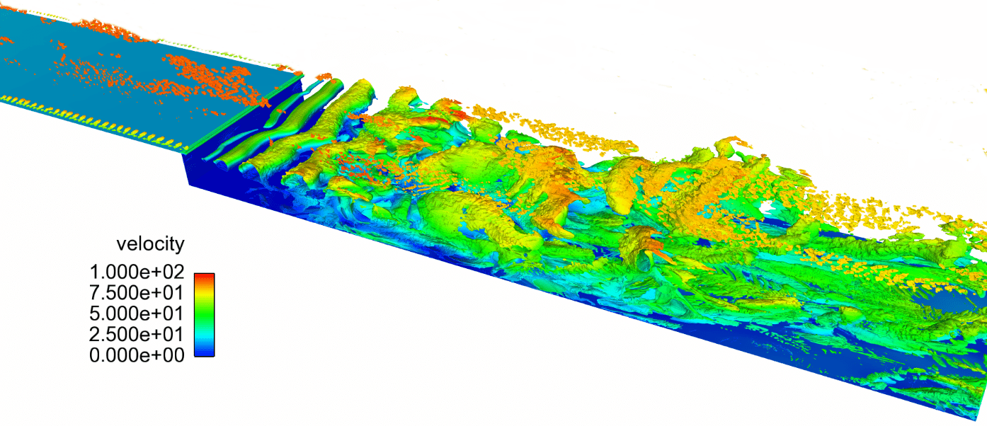
Detached Eddy Simulation (DES) is a hybrid model, taking advantage of the similarity of functional forms of the turbulent viscosities in RANS and LES. DES adopts RANS-like behavior near the wall, where we know an LES can be very computationally expensive. DES adopts LES behavior far from the wall, where LES is more computationally tractable and unsteady turbulent motions are more often important.

The math behind this switching behavior is beyond the scope of a blog post. In effect, DES solves the Navier-Stokes equations with some effective \({\mu _{t,DES}}\) such that \({\mu _{t,DES}} \approx {\mu _{t,RANS}}\) near the wall and \({\mu _{t,DES}} \approx {\mu _{t,LES}}\) far from the wall, with \({\mu _{t,RANS}}\) and \({\mu _{t,LES}}\) selected and tuned so that they are compatible in the transition region. Our understanding of the derivation and characteristics of the RANS and LES turbulence models allows us to hybridize them into something new.

*This term is a symmetric second-order tensor, so it has six scalar components. In some approaches (e.g., Reynolds Stress models), we might transport these terms separately, but the eddy viscosity approach treats this unknown tensor as a scalar times a known tensor.